Semantic Understanding of Dermatology Images Using LLaVA and RAG

Overview

In this blog entry, we will explain how to bridge the gap between patients and accessible, accurate dermatological consultations by leveraging advanced Vision-Language Models (VLMs). Given the rise in demand for reliable and immediate medical advice, particularly in dermatology, this tool empowers users to consult an “online dermatologist” by providing essential information, an image of the affected area, and asking follow-up questions, closely mimicking an actual consultation. This tool can also potentially assist medical practitioners as a preliminary diagnostic aid.

To achieve this, we fine-tuned a domain-specific Language and Vision Assistant (LLaVA) model, equipping it with the ability to process and analyze user-provided images, such as those of rashes, inflammations, or other skin conditions, and give patients diagnoses with high accuracy. By integrating Retrieval-Augmented Generation (RAG) as well, this pipeline significantly mitigates hallucination, making its responses highly reliable for medical inquiries which is crucial in the medical domain. Dermatologists have validated the responses as “solid” in clinical accuracy, indicating the model’s practical relevance for real-world medical applications.

We also provide a detailed LLaVA architecture tutorial with the hope to help our readers gain a deeper understand the LLaVA architecture and make necessary modifications to suit their own applications.

We hope our model allows allows researchers, developers, and healthcare providers to experiment, refine, and extend its capabilities. It opens possibilities for broader healthcare applications and innovations while fostering transparency and collaboration in AI-driven medical tools. You can find our finetuned model on our Huggingface.

Overall Impact

Primary Issues Addressed

A key issue this project addresses is the accessibility of dermatological consultation. Traditional consultations typically require in-person visits, often resulting in long wait times and significant costs. This model aims to democratize access by allowing patients to receive basic advice without the need for immediate clinic access, which is especially valuable for individuals in remote or underserved areas.

Another major concern is the issue of medical hallucination in AI models. Many language models (LLMs) exhibit hallucination, particularly in sensitive fields like healthcare. To mitigate this, we implemented Retrieval-Augmented Generation (RAG), where the model retrieves relevant information before generating responses. By comparing three different RAG methods, we ensure that responses are based on reliable sources, reducing the risk of errors in medical advice.

Lastly, we address the scarcity of specialized AI models in healthcare. While generic AI models are widely available, there is a limited number of finely-tuned, specialized models for healthcare applications. Our model is specifically trained for dermatology, incorporating real feedback from dermatologists, thus ensuring a high standard of accuracy and usability for both clinical and personal use.

Project Pipeline

Overview of Training/Validation Data Set

Google Research released the Skin Condition Image Network (SCIN) dataset in collaboration with physicians at Stanford Medicine. SCIN is designed to reflect the broad range of concerns that people search for online, supplementing the types of conditions typically found in clinical datasets. The data is stored in the dx-scin-public-data bucket on Google Cloud Storage.

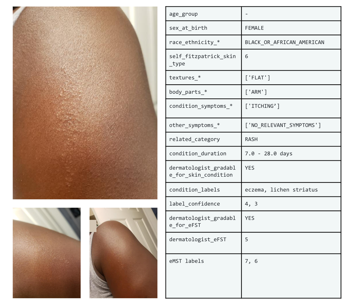
Figure 1: Example of SCIN dataset

The SCIN open access dataset contains more than 10k images of common dermatology conditions (5,000+ volunteer contributions). Meanwhile, self-reported demographic, history, and symptom information, and self-reported Fitzpatrick skin type (sFST), dermatologist labels of the skin condition and estimated Fitzpatrick skin type (eFST) and layperson estimated Monk Skin tone (eMST) labels are provided for each contribution.

Diagnosis Process

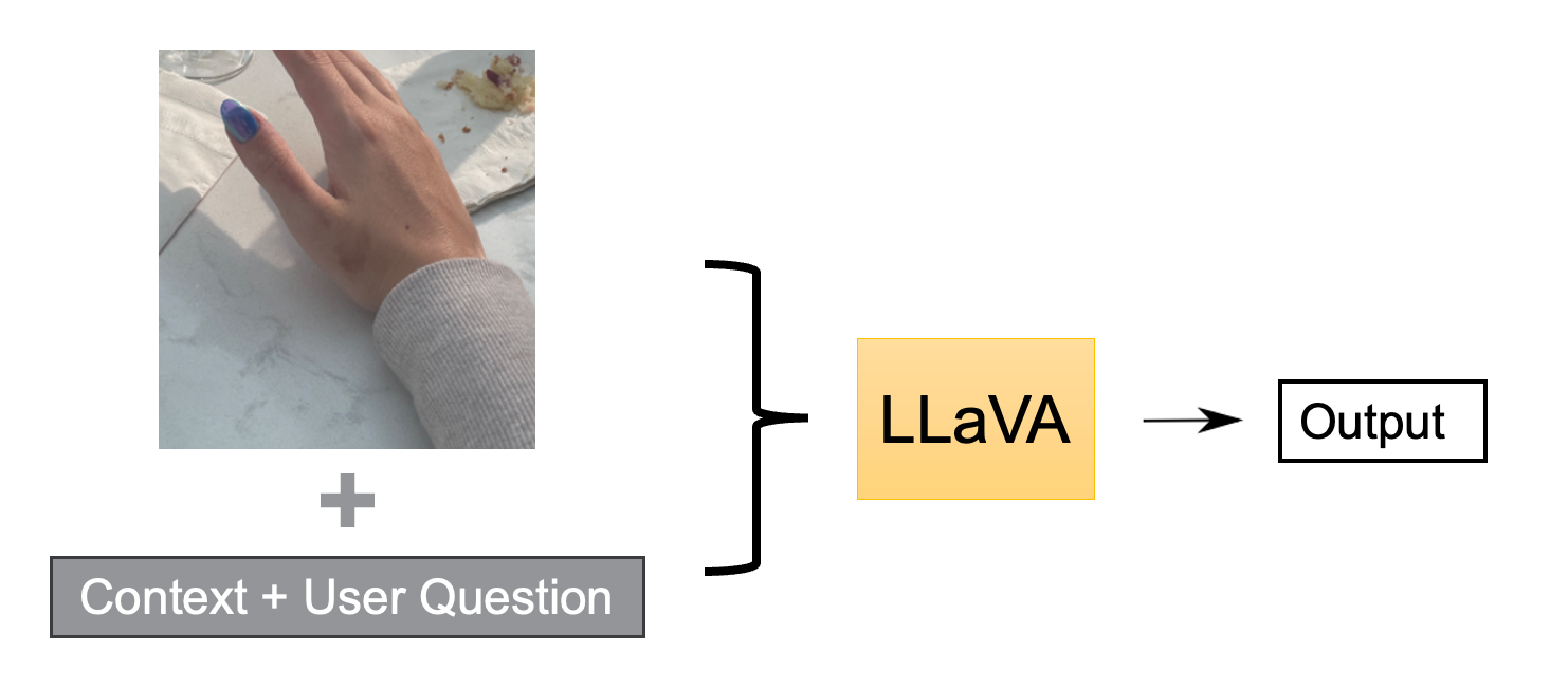
Figure 2: MLLM Diagnosis with Background Information and Images

In the first part of our tool, patients can provide essential information and an image of the affected area, closely mimicking an actual consultation. The model is trained to return diagnosis with corresponding probabilities.

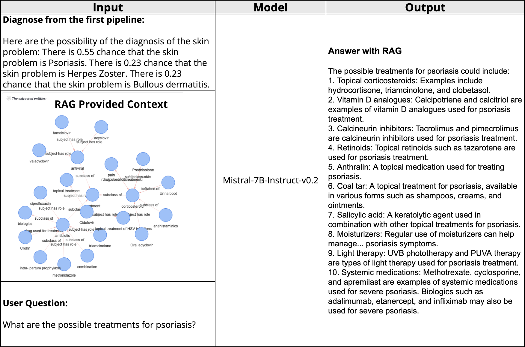
Follow-up Question Regarding the Diagnosis

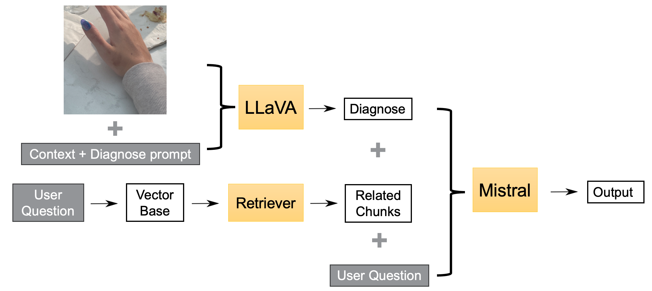
Figure 3: LLM Answering Follow-Up Questions

To enhance the tool’s ability to further answer detailed questions, we utilized the strength of Mistral for dealing with longer context. With RAG retrieved context providing solid truth and diagnosis from the first section, only text input is fed into Mistral for the patient’s further questions.

Training

Data Preprocessing

The dataset contains contributions from 5k volunteers, each providing 1-3 images from AT_AN_ANGLE, CLOSE_UP, AT_DISTANCE, adding up to 10k images. 39% and 55% of volunteers did not provide a second or a third picture, respectively.

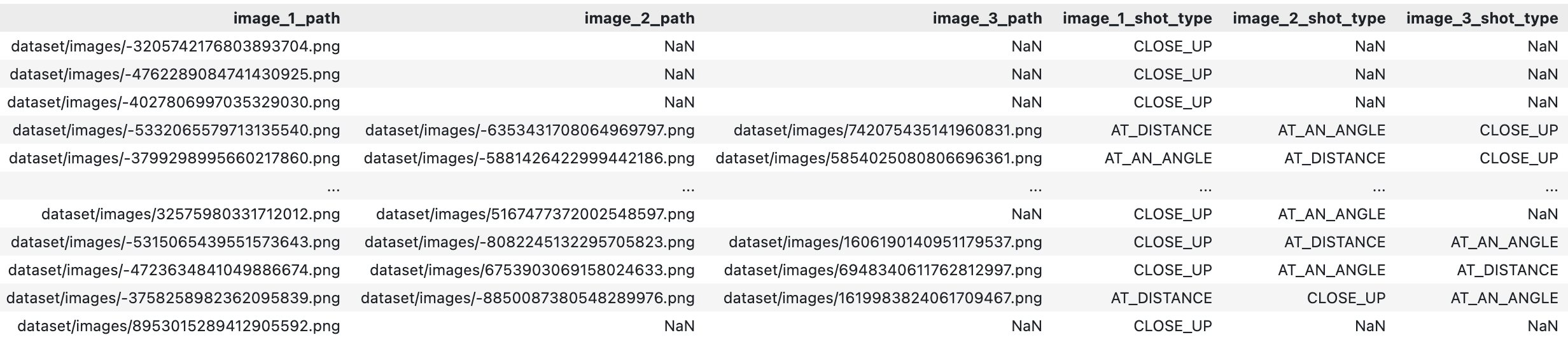
Figure 4: Missing Values in the Dataset

Due to space constraints, we will skip most of the common data preprocessing steps, and focus on how we deal with the missing data.

For CLOSE_UP image missing, we used Object Detection Models (YOLOv3) to return the bounding box of human bodies and clipped the image to make a CLOSE_UP version.
For missing numerical features, we used interpolation to estimate values between known data points, ensuring smoother transitions and continuity. In cases where interpolation wasn’t applicable, we applied forward and backward filling to propagate adjacent values, maintaining temporal consistency where appropriate.
For missing categorical data, we imputed missing values by assigning the most frequent category or using domain-specific assumptions.

Data Forming

To make the best use of the dataset, we construct a context of patient information based on every feature:

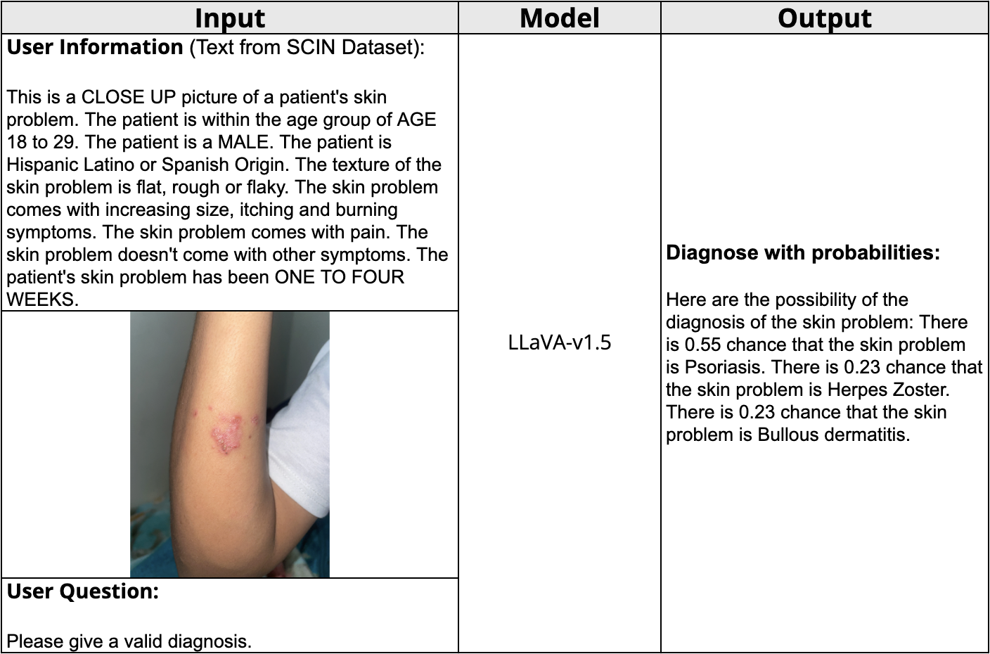
This is a CLOSE UP picture of a patient’s skin problem. The patient is within the age group of AGE 18 TO 29. The patient is a MALE. The patient is Hispanic Latino or Spanish Origin. The texture of the skin problem is flat, rough or flaky. The skin problem comes with increasing size, itching, burning symptoms. The skin problem comes with pain. The skin problem doesn’t come with other symptoms. The patient’s skin problem has been ONE TO FOUR WEEKS.

Code-level Explanation of LLaVA's Model Structure

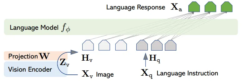
Figure 5: LLaVA Architecture

As a state-of-the-art multi-modal language model (MLLM), LLaVA-v1.5 excels in visual understanding and can be further optimized for specific domains through fine-tuning. Our initial step involved restructuring the LLaVA pipeline to support research applications.

The LLaVA model architecture is comprised of three main components: (1) CLIP, which generates the visual representation; (2) the Multi-modal Projector, which maps this visual representation into the language latent space; and (3) the Large Language Model, which performs question-answering based on the image content.

Load LLaVA and Split Into 3 Parts

from transformers import LlavaForConditionalGeneration
llava = LlavaForConditionalGeneration.from_pretrained(
    "llava-hf/llava-v1.6-vicuna-7b-hf", 
    torch_dtype=torch.float32, 
    device_map = 'auto', 
)
# Save Separately
torch.save(llava.vision_tower, './vision_tower.pt')
torch.save(llava.multi_modal_projector, './multi_modal_projector.pt')
torch.save(llava.language_model, './language_model.pt')

Step 1: With a clear LLaVA pipeline in place, we can now begin developing our own code. The first step is to load the individual model components and obtain the prompt embeddings.

Load Model Parts Separately

from transformers import AutoTokenizer,AutoImageProcessor
from PIL import Image
from transformers.models.auto.configuration_auto import CONFIG_MAPPING

# Step1: Load Everything in 16
device = 'cuda:1'

vision_tower = torch.load('./vision_tower.pt').to(device, torch.float16)
image_processor = AutoImageProcessor.from_pretrained("llava-hf/llava-v1.6-vicuna-7b-hf")
multi_modal_projector = torch.load('./multi_modal_projector.pt').to(device, torch.float16)
language_model = torch.load('./language_model.pt').to(device, torch.float16)
tokenizer = AutoTokenizer.from_pretrained("llava-hf/llava-v1.6-vicuna-7b-hf")

Step 2: We designate the position of the image in the prompt by adding <image>, which LLaVA’s tokenizer recognizes as image_token_index = 32000. However, before passing input_ids to the Vicuna model to obtain input_embeddings, we replace this index with 0 to ensure correct processing.

Extract Prompt Embeddings

# Set configurations
image_token_index = 32000
image_grid_pinpoints = [[336, 672], [672, 336], [672, 672], [1008, 336], [336, 1008]]
vision_config = CONFIG_MAPPING["clip_vision_model"](intermediate_size=4096, hidden_size=1024, patch_size=14, image_size=336, num_hidden_layers=24, num_attention_heads=16, vocab_size=32000, projection_dim=768,)

# Step2: Extract the Prompt embeddings
prompt = "USER: <image>\n The patient's fitzpatrick skin type is Type IV, which means burns minimally, always tans well (moderate brown). . The patient is American Indian or Alaska native. The texture of the skin problem is raised or bumpy.  The skin problem comes with itching symptoms. The skin problem doesn't come with other symptoms. The patient's skin problem has been MORE THAN ONE YEAR.Please give a valid diagnose.\nASSISTANT:"
input_ids = tokenizer(prompt, return_tensors='pt')['input_ids'].to(device)
attention_mask = tokenizer(prompt, return_tensors='pt')['attention_mask'].to(device)
for_inputs_embeds_ids = input_ids.clone()
for_inputs_embeds_ids[(input_ids == image_token_index)] = 0
inputs_embeds = language_model.get_input_embeddings()(for_inputs_embeds_ids)

Step 3: As shown in the LLaVA architecture in Figure 5, we use the vision tower to obtain the image features and prepare it for projection. Specifically, we are taking the hidden states from the specific vision feature layer(-2) and removing the first embedding of the selected features, since we set vision_feature_select_strategy = "default".

Core Code of Get Image Embedding

# Step3: Getting Image Feature
Image_path = YOUR_IMAGE_PATH
images = Image.open(Image_path).convert('RGB')
pixel_values = image_processor(images, return_tensors='pt')["pixel_values"][0].to(device)

# -2 is the original llava config
vision_feature_layer = -2
image_features = vision_tower(pixel_values, output_hidden_states=True)
selected_image_feature = image_features.hidden_states[vision_feature_layer]
# Using the default vision feature select strategy, drop first embeddings
selected_image_feature = selected_image_feature[:, 1:]

The vision_feature_select_strategy parameter determines how visual features are selected from the vision backbone for further processing. It has two options:

"default" Strategy: In this mode, the CLS token is removed from the vision features. The CLS token typically serves as a summary representation of the entire image, but excluding it means that only the patch embeddings (representations of image segments) are utilized. This approach focuses on detailed, localized information from the image.
"full" Strategy: Here, the full set of vision features is used, including the CLS token. This means both the global summary (CLS token) and the detailed patch embeddings are considered, providing a comprehensive representation of the image.

Step 4: After obtaining the text and image embeddings, we need to transform them into the same latent space. Please notice that the number of patches (image_num_patches) was calculated in Step 3, and this is applied along dimension 0. You can find the process of defining image_num_patches in our full script at the end of this section.

Projection

# Step4: Project from image to language representation
image_features = multi_modal_projector(selected_image_feature)
image_features = torch.split(image_features, image_num_patches, dim=0)

Step 5: Within this step, we will need to reshape, unpad and then pack each image_feature into a single image_features tensor containing all visual vectors, aiming to prepare the processed image features for merging with text embeddings.

We’ll borrow two pre-defined functions from Transformer llava_next github repo: unpad_image and pack_image_features.

unpad_image function removes padding from the image tensor to return it to its original aspect ratio.
pack_image_features function prepares image features by reshaping and packing into a unified tensor structure. The output includes the packed image_features tensor and feature_lens, which keeps track of the length of features for each image.

Pack Image Features

# Step5: Prepare image features for merging
# Reshape, unpad and then pack each image_feature into a single image_features tensor containing all visual vectors
image_features, feature_lens = pack_image_features(
                    image_features,
                    image_sizes = [image_sizes],
                    image_newline=None,
                )

This step ensures that the visual data remains structured and accessible for further merging.

Step 6: Now we need to merge the text and image features and fill the embeddings based on the mask:

We borrow the function _merge_input_ids_with_image_features from LLaVA’s official repo, which populates the final embeddings based on text and image’s respective positions and ensures alignment. Here is an example:

Example:
If we have [‘this’, ‘<image>’, ‘is’, ’a’, ‘trial’], we need to index copy on [0, 577, 578, 579, 580] for the text and [1:576] for the image features

Merge Text and Image Features

def _merge_input_ids_with_image_features(image_features, feature_lens, inputs_embeds, input_ids, attention_mask, position_ids=None, labels=None, image_token_index=None, ignore_index=-100,):
        image_token_index = 32000
        ignore_index = ignore_index

        with torch.no_grad():
            num_images = feature_lens.size(0)
            num_image_features, embed_dim = image_features.shape
            if feature_lens.sum() != num_image_features:
                raise ValueError(f"{feature_lens=} / {feature_lens.sum()} != {image_features.shape=}")
            batch_size = input_ids.shape[0]
            _left_padding = torch.any(attention_mask[:, 0] == 0)
            _right_padding = torch.any(attention_mask[:, -1] == 0)

            left_padding = True
            if batch_size > 1:
                if _left_padding and not _right_padding:
                    left_padding = True
                elif not _left_padding and _right_padding:
                    left_padding = False
                elif not _left_padding and not _right_padding:
                    left_padding = True
                else:
                    # invalid attention_mask
                    raise ValueError(f"both side of attention_mask has zero, invalid. {attention_mask}")
            
            # Whether to turn off right padding
            # 1. Create a mask to know where special image tokens are
            special_image_token_mask = input_ids == image_token_index
            num_special_image_tokens = torch.sum(special_image_token_mask, dim=-1)
            # Reserve for padding of num_images
            total_num_special_image_tokens = torch.sum(special_image_token_mask)
            if total_num_special_image_tokens != num_images:
                raise ValueError(
                    f"Number of image tokens in input_ids ({total_num_special_image_tokens}) different from num_images ({num_images})."
                )
            # Compute the maximum embed dimension, max_image_feature_lens is max_feature_lens per batch
            feature_lens = feature_lens.to(input_ids.device)
            feature_lens_batch = feature_lens.split(num_special_image_tokens.tolist(), dim=0)
            feature_lens_batch_sum = torch.tensor([x.sum() for x in feature_lens_batch], device=input_ids.device)
            embed_sequence_lengths = (
                (attention_mask == 1).long().sum(-1) - num_special_image_tokens + feature_lens_batch_sum
            )
            max_embed_dim = embed_sequence_lengths.max()
            batch_indices, non_image_indices = torch.where((input_ids != image_token_index) & (attention_mask == 1))
            # 2. Compute the positions where text should be written
            special_image_token_mask = special_image_token_mask.long()
            special_image_token_mask[special_image_token_mask == 1] = feature_lens - 1
            new_token_positions = torch.cumsum((special_image_token_mask + 1), -1) - 1
            if left_padding:
                new_token_positions += max_embed_dim - 1 - new_token_positions[:, -1:]

            text_to_overwrite = new_token_positions[batch_indices, non_image_indices]

        # 3. Create the full embedding, already padded to the maximum position
        final_embedding = torch.zeros(
            batch_size, max_embed_dim, embed_dim, dtype=inputs_embeds.dtype, device=inputs_embeds.device
        )
        final_attention_mask = torch.zeros(
            batch_size, max_embed_dim, dtype=attention_mask.dtype, device=inputs_embeds.device
        )
        final_input_ids = torch.full(
            (batch_size, max_embed_dim), pad_token_id, dtype=input_ids.dtype, device=inputs_embeds.device
        )
        # Double check: set the corresponding tensors into their correct target device.
        target_device = inputs_embeds.device
        batch_indices, non_image_indices, text_to_overwrite = (
            batch_indices.to(target_device),
            non_image_indices.to(target_device),
            text_to_overwrite.to(target_device),
        )
        attention_mask = attention_mask.to(target_device)
        input_ids = input_ids.to(target_device)

        # 4. Fill the embeddings based on the mask.
        final_embedding[batch_indices, text_to_overwrite] = inputs_embeds[batch_indices, non_image_indices]
        final_attention_mask[batch_indices, text_to_overwrite] = attention_mask[batch_indices, non_image_indices]
        final_input_ids[batch_indices, text_to_overwrite] = input_ids[batch_indices, non_image_indices]
        final_labels = None
        if labels is not None:
            labels = labels.to(target_device)
            final_labels = torch.full_like(final_attention_mask, ignore_index).to(torch.long)
            final_labels[batch_indices, text_to_overwrite] = labels[batch_indices, non_image_indices]

        # 5. Fill the embeddings corresponding to the images. Anything that is not `text_positions` needs filling (#29835)
        with torch.no_grad():
            image_to_overwrite = torch.full(
                (batch_size, max_embed_dim), True, dtype=torch.bool, device=inputs_embeds.device
            )
            image_to_overwrite[batch_indices, text_to_overwrite] = False
            embed_indices = torch.arange(max_embed_dim).unsqueeze(0).to(target_device)
            embed_indices = embed_indices.expand(batch_size, max_embed_dim)
            embed_seq_lens = embed_sequence_lengths[:, None].to(target_device)

            if left_padding:
                # exclude padding on the left
                max_embed_dim = max_embed_dim.to(target_device)
                val = (max_embed_dim - embed_indices) <= embed_seq_lens
            else:
                # exclude padding on the right
                val = embed_indices < embed_seq_lens
            image_to_overwrite &= val

            if image_to_overwrite.sum() != num_image_features:
                raise ValueError(
                    f"{image_to_overwrite.sum()=} != {num_image_features=} The input provided to the model are wrong. "
                    f"The number of image tokens is {torch.sum(special_image_token_mask)} while"
                    f" the number of image given to the model is {num_images}. "
                    f"This prevents correct indexing and breaks batch generation."
                )
        final_embedding[image_to_overwrite] = image_features.contiguous().reshape(-1, embed_dim).to(target_device)
        final_attention_mask |= image_to_overwrite
        position_ids = (final_attention_mask.cumsum(-1) - 1).masked_fill_((final_attention_mask == 0), 1)

        return final_embedding, final_attention_mask, position_ids, final_labels, final_input_ids

# Step6: Merge the text and image features
position_ids = None
inputs_embeds, attention_mask, position_ids, labels, _ = _merge_input_ids_with_image_features(
                    image_features,
                    feature_lens,
                    inputs_embeds,
                    input_ids,
                    attention_mask,
                    position_ids,
                    labels=input_ids,
                )

Step 7: Once we have the final merged representation, we can use it as input for the LLM to perform the final QA inference.

LLM Inference

# Step7: Using language_model to get the output
past_key_values = None
use_cache = None
output_attentions = None
output_hidden_states = None
return_dict = None
max_new_tokens = 128
with torch.no_grad():
    generated_ids = []
    for _ in range(max_new_tokens):
        outputs = language_model(
            attention_mask=attention_mask,
            position_ids=position_ids,
            past_key_values=past_key_values,
            inputs_embeds=inputs_embeds,
            use_cache=use_cache,
            output_attentions=output_attentions,
            output_hidden_states=output_hidden_states,
            return_dict=return_dict,
        )
        logits = outputs[0]
        next_token_logits = logits[:, -1]
        index_pred = torch.argmax(next_token_logits, -1)
        generated_ids.append(index_pred.item())
        inputs_embeds = torch.concat([inputs_embeds, language_model.get_input_embeddings()(index_pred).unsqueeze(0)], 1)
        attention_mask = torch.concat([attention_mask, torch.ones(1, device=attention_mask.device).unsqueeze(0)], 1)
        position_ids = torch.concat([position_ids, torch.tensor(position_ids[:,-1]+1, device=position_ids.device).unsqueeze(0)], 1)

print(tokenizer.decode(generated_ids))

We hope this detailed tutorial helps our readers gain a deeper understanding of the LLaVA architecture and make necessary modifications to suit their own applications. For the dermatology user case, we applied LoRA technique to all linear layers in CLIP and LLM. Fine tuning was conducted on 2 A100 80G cards with lora settings “lora_r 32 --lora_alpha 64“, and our trainable parameters were kept to under 1% of the base model size.

RAG

Introduction

We explore three unique types of RAG: Knowledge Graph RAG, Flat Index RAG and HyDE RAG—each leveraging different methods for retrieval and augmentation to address specific challenges in real-world applications. While all methods enhanced the model’s capabilities, our results showed that the Knowledge Graph RAG outperformed FAISS IndexFlat, particularly in providing contextually accurate and medically reliable answers.

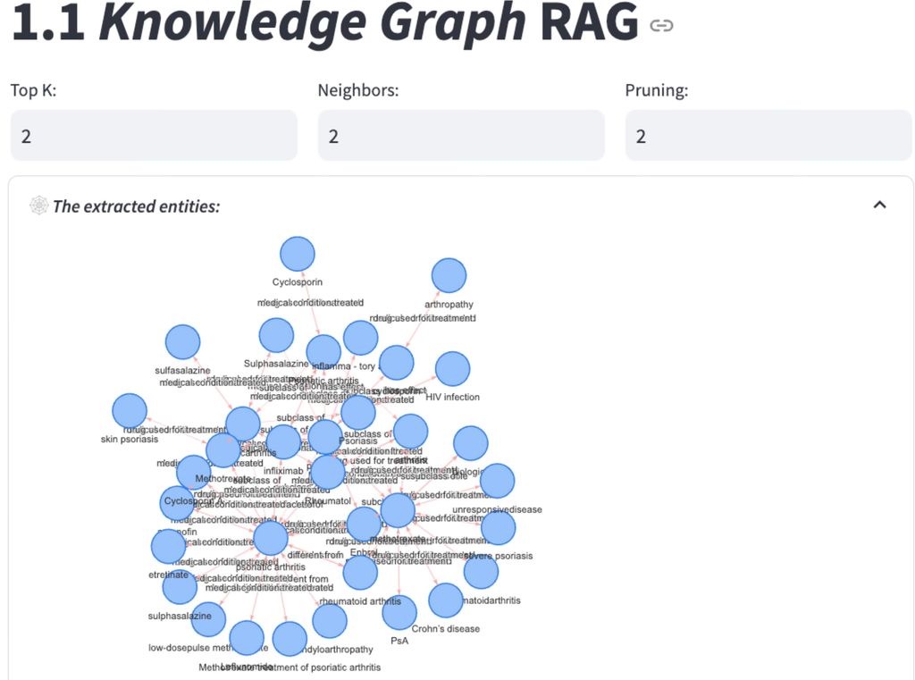
Knowledge Graph RAG (KGRAG)

Knowledge Graph RAG stands out by employing structured data in the form of knowledge graphs, where entities and relationships provide contextualized, interconnected information. It retrieves relevant nodes and edges from a knowledge graph, offering a detailed and precise context that is highly suitable for complex applications, such as medical diagnoses or expert systems. By utilizing structured, domain-specific knowledge, KGRAG is able to return cross-document information (compared to other methods that can only return several full chunks, KGRAG can extract relevant triplets grounded in verified relationships from hundreds of chunks).

Flat Index RAG

Flat Index RAG utilizes a simple but efficient approach to retrieve data points based on vector similarity, often leveraging libraries like FAISS to index and retrieve embeddings. In this method, a “flat” or unstructured index is created, enabling fast and scalable retrieval of similar items based on vector distance. Flat Index RAG is particularly effective in applications where low-latency retrieval is crucial and the data set is relatively simple, such as FAQ or product recommendation systems. Our findings indicated that FAISS IndexFlat lacks some of the nuanced, relational depth achieved with the Knowledge Graph approach.

HyDE RAG

HyDE is inspired by the paper “Precise Zero-shot Dense Retrieval without Relevance Labels”. It takes a unique approach by generating a hypothetical passage to enhance retrieval. This model creates potential answers or explanations, embeds them into the vector space, and retrieves them based on relevance to a given query. We found HyDE RAG is especially useful in scenarios where the user question is general and simple, using the hypothetical answer for retrieval will return more relevant chunks from our data base.

Building the Database

To power both RAG methods, we collected more than 700 dermatology-related terms, and built a comprehensive dataset with over 8k articles by collecting open access materials from two platforms:

Wikipedia: We retrieved the wiki page for each medical term, along with the top 5 related wiki pages found through searches of the medical term.

PubMed: We accessed the most relevant articles (with CC0, CC BY, CC BY-SA, CC BY-ND licenses) for each keyword through E-utilities , which is the official method of collecting data from NCBI (National Center for Biotechnology Information).

This dataset, rigorously curated for dermatology-related content, served as the foundation for all three RAG methods mentioned above.

RAG Retrieval Evaluation

1. Retrieved Content Quailty

For example, if a patient query involves “symptoms”, the Knowledge Graph helps the model not only retrieve related conditions, such as eczema or psoriasis, but also the relationships between these conditions, including treatment options and diagnostic pathways. This depth in relational data allows the model to produce responses that more closely mirror the reasoning process a dermatologist might follow, adding a level of context that enhances response accuracy.

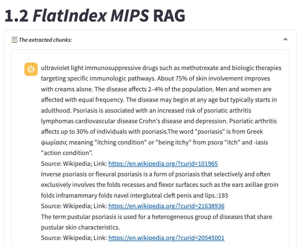
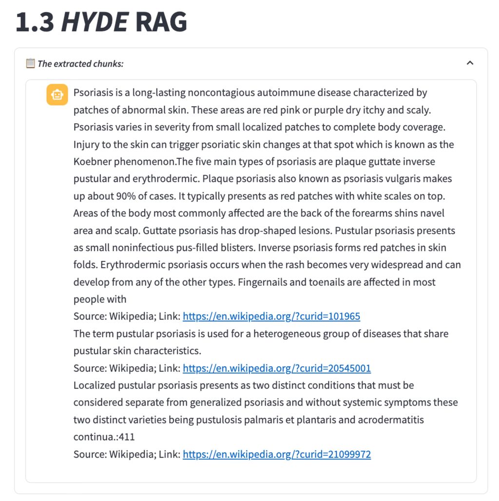
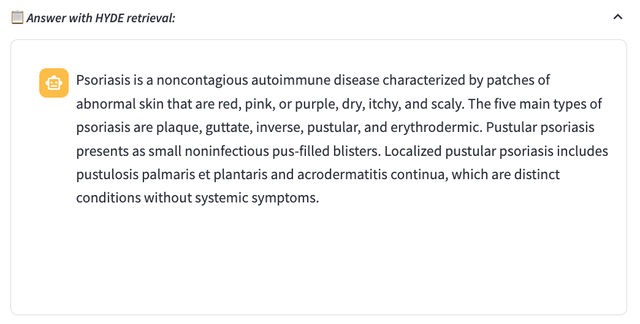
The FlatIndex and HYDE methods often return general introductions to the term ‘Psoriasis’ along with information on various psoriasis syndromes. This can introduce extra, irrelevant information, potentially leading to hallucinations in the LLM, which tends to rely heavily on the provided context.

2. Retrieval Speed

Method	Average Retrieval Time
KGRAG	0.31 sec
FlatIndex RAG	0.02 sec
HyDE RAG	9.67 sec

HyDE requires the LLM to generate an answer first, which is then used for retrieval, significantly increasing the overall processing time. Meanwhile, the FlatIndex from FAISS library performs optimally, adding minimal latency to the entire pipeline.

3. Real World Validation

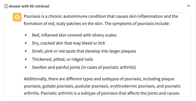
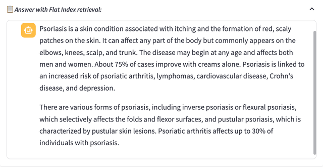
Above are some examples of LLM responses to the question, “What are the symptoms of psoriasis?” provided with different contexts from KGRAG, FlatIndex RAG, and HyDE RAG. Thanks to the high quality of content retrieved by KGRAG, KGRAG + LLM provides the most accurate answer, effectively reducing hallucinations and delivering highly relevant and reliable results.

Practicing dermatologists evaluated our model’s output, confirming that the responses generated via the Knowledge Graph RAG approach aligned closely with established dermatological practices. This validation reinforces the model’s clinical reliability, indicating that Knowledge Graph RAG, in particular, provides an effective and dependable solution for medical AI applications in dermatology.

Inferencing in ET-SoC-1

Figure 6: Demo Running on ET-SoC-1

We built the webpage based on a Streamlit package, and it is running on Esperanto’s ET-SoC-1 chip. The above video shows a complete example of patient consulting our Dermatology Diagnosis AI.