Problem Definition
Minimally invasive and robotic-assisted surgeries have revolutionized the field of surgery, enabling precision and reducing patient recovery time. However, a major challenge in analyzing and learning from surgical videos is the occlusion caused by surgical instruments and the patches of blood coming from hemorrhages, which can obscure critical anatomical structures. This limits the ability of surgeons, AI-assisted systems, and medical trainees to fully understand intraoperative events.
In recent years, computer vision and deep learning have significantly advanced surgical video analysis, with segmentation and inpainting techniques playing a crucial role. Segmenting surgical tools and blood occlusions is a key step toward reconstructing the hidden anatomical structures underneath, allowing for better surgical AI training, intraoperative assistance, and post-operative analysis.
To address this, we propose an end-to-end pipeline that segments, inpaints, and enhances surgical video frames, offering a clearer view of the operating field. Our method leverages SAM2 (Segment Anything Model v2) for high-precision segmentation of tools and blood, followed by ProPainter for realistic inpainting, effectively predicting the underlying structures. Additionally, we integrate signal processing and post-processing techniques to enhance visual clarity, particularly in addressing motion blur and artifacts. Furthermore, we incorporate measurement techniques for tool movement and depth analysis, adding a layer of quantitative insight into surgical tool dynamics.
Contribution
Our work introduces a novel segmentation-inpainting pipeline specifically designed for surgical video analysis, with the following key contributions:
1. High-Precision Segmentation of Surgical Tools and Blood Using SAM2
We employ SAM2 to achieve accurate instance segmentation of surgical tools and blood occlusions in real-time. This enables precise identification of obstructed regions, paving the way for reliable inpainting.
2. Instrument and Hemorrhage Removal via ProPainter-Based Inpainting
Using ProPainter, we predict and restore the hidden anatomical structures under instruments and blood, providing a clearer visual representation of the surgical field.
3. Post-Processing with Signal Processing & Deblurring Intuitions
We explore and tune ProPainter hyperparameters to enhance inpainting stability and realism. To further refine the results, we integrate signal processing techniques, particularly in cases where surgical video frames suffer from motion blur. Our deblurring process enhances frame quality and temporal consistency, aiding AI-based surgical video analysis.
4. Quantitative Measurement of Surgical Tool Movement and Depth
We introduce motion tracking and depth estimation for surgical tools, providing quantitative metrics on tool movement dynamics. This data can be leveraged for surgical skill assessment, robotic surgery optimization, and AI-assisted surgery planning.
5. A Comprehensive, Open-Source Framework for Surgical Video Enhancement
Our work provides a modular and scalable pipeline, allowing future researchers and medical professionals to apply or extend our methodology. We ensure that our segmentation-inpainting-deblurring approach is generalizable, making it applicable to a wide range of surgical specialties and video conditions.
Proposed Solution
Automation for surgery has progressed across multiple disciplines to tackle the wide variety of surgical tasks including Augmented Reality (AR) for intuitive visual cues, robotic systems that surgeons operate with, and video analysis for post-operation review. Even with the significant progress found in automation for surgery, the crucial surgical task of hemostasis management, the process of managing and controlling bleeding during surgery such that there are no occlusions from blood, has not received much attention. Hemorrhaging occurs in surgeries of all types, forcing surgeons to quickly adapt to the visual interference that results from blood rapidly filling the surgical field and establish hemostasis as quickly as possible to minimize bleeding and allow the critical tasks of the operation to proceed.
Significant instrumentation and tools have been designed for surgeons to control bleeding (e.g. cautery, staplers, sutures), since the surgical task of maintaining hemostasis is universal to all surgeries. However, automation efforts in hemostasis management have been limited to only a few works, all of which directly avoid the challenge of segmenting blood from surgical cameras via image classification (blood or no blood), namely event-based detection of active bleeding and automation of the suction tool to remove blood, hand-crafted optical flow filtering, color-based detection in a lab bench-top setting, and over-fitting to the specific lab bench-top setting.
We choose HemoSet as our testing dataset, the first to feature segmented blood in a surgical setting, addressing the need for labeled data that is representative of the domain. We highlight the key challenges of this dataset as follows: 1) erratic pooling geometry: the turbulent nature of the environment causes unique contours with each incision, 2) distinction of pools and stains: they are categorically distinct relative to hemostasis despite their visual similarity, and 3) varying difficulty: the variety of incisions and pool contours ensure novel difficulty levels across different segments of the video. We believe that our dataset will be a valuable resource for researchers and developers working on automatic hemostasis algorithms and systems.
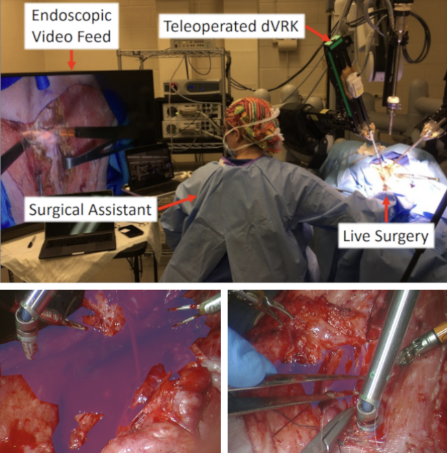
Figure 1: HemoSet Example
Pipeline Overview
We split the current task into Segmentation, Tracking and Inpainting, and for this project we also provide the exploration for deblurring and measurement.
| Segmentation | Tracking | Inpainting | Deblurring | Measurement | ||
| Text Prompt | Pointer Prompt | Reference Image | Post-Processing | |||
| YOLOv8+SAM2 | SAM2 | SAM2 | Propainter | Change Propainter List | Signal Processing | Movement and Depth |
Figure 2: Pipeline Overview
Segmentation: SAM2
SAM2 is an upgraded version of SAM, designed to deliver high-precision, prompt-based segmentation across various fields, including medical imaging, autonomous driving, and robotic vision. Developed by Meta AI, SAM2 enhances its predecessor by offering greater accuracy, efficiency, and adaptability, making it well-suited for complex segmentation challenges.
Unlike conventional segmentation models that require task-specific training, SAM2 is designed to generalize. With minimal supervision, it can adapt to new objects and images, making it an invaluable tool for applications where segmentation masks must be generated on demand.
SAM2 starts by processing user prompts and generates dynamic masks. Utilizing self-attention mechanisms and transformer-based feature extraction, SAM2 adjusts its mask predictions based on the surrounding context. Compared to earlier versions, it reduces false positives and enhances edge precision, ensuring more reliable segmentation. Moreover, a final context-aware optimization step refines the mask, ensuring higher segmentation accuracy and well-defined object boundaries.
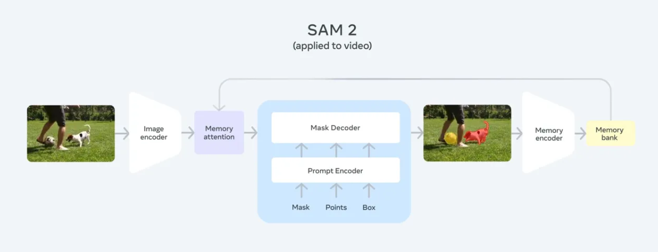
Figure 3: SAM2 Structure Overview
In our project, SAM2 plays a critical role in segmenting surgical tools and blood areas in real-time surgical videos. It generates highly accurate masks and ensures clean segmentation boundaries for reconstructing hidden anatomical structures. To make our project adaptable to real-world operating room conditions, SAM2 was also used for handling dynamic movements and keeping track of the selected areas. Followed are two examples of SAM2’s performance in tracking all instruments in a surgical video:
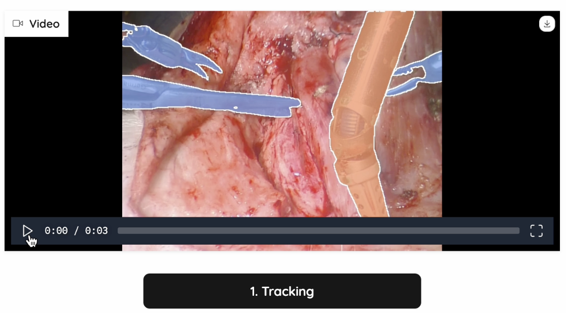
Figure 4: Tracking Example 1
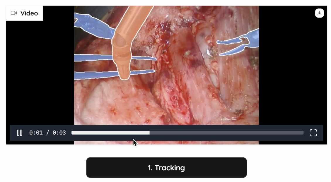
Figure 5: Tracking Example 2
With our user interface, we can provide pointers into the SAM2 model using a simple click, indicating the area of which entity we want to do segmentations on.
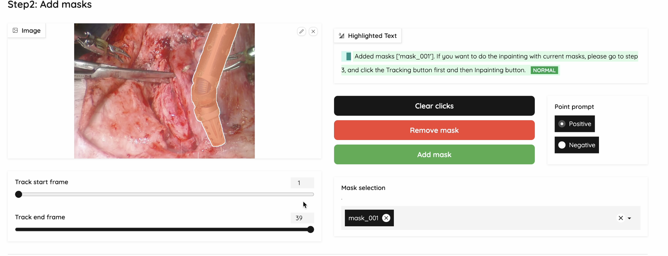
Figure 6: Segmentation UI Example
Here are the functions we provide in our web UI:
-
Show Current Mask: Click on the image and immediately shows the corresponding mask
-
Add Multiple Masks: We are able to save each mask and let users select multiple masks for the next step
-
Negative and Positive Prompts: Used for generating a fine-grained mask
-
Clear Clicks: Clear clicks on the current frame
-
Validate & Run Inpainting: Used to start inpainting with the selected masks
Inpainting: ProPainter
We have tested out multiple models on video-inpainting tasks (Stable-diffusion-video, Inpainting-Anything, Realfill, etc.) We found two benchmarks and adapted the SOTA model: ProPainter: Improving Propagation and Transformer for Video Inpainting. It is able to utilize the spatial, temporal and optical information, and search for the most similar patches as reference, to generate trustworthy and high quality inpainted videos.
The inpainting will be quite accurate from masked pixels that are visible in other frames if the data is available, or it will make a best guess from surrounding pixels, if the correct masked pixels are not available. On the inpainting video, the thin contours of the inpainting regions will be shown.
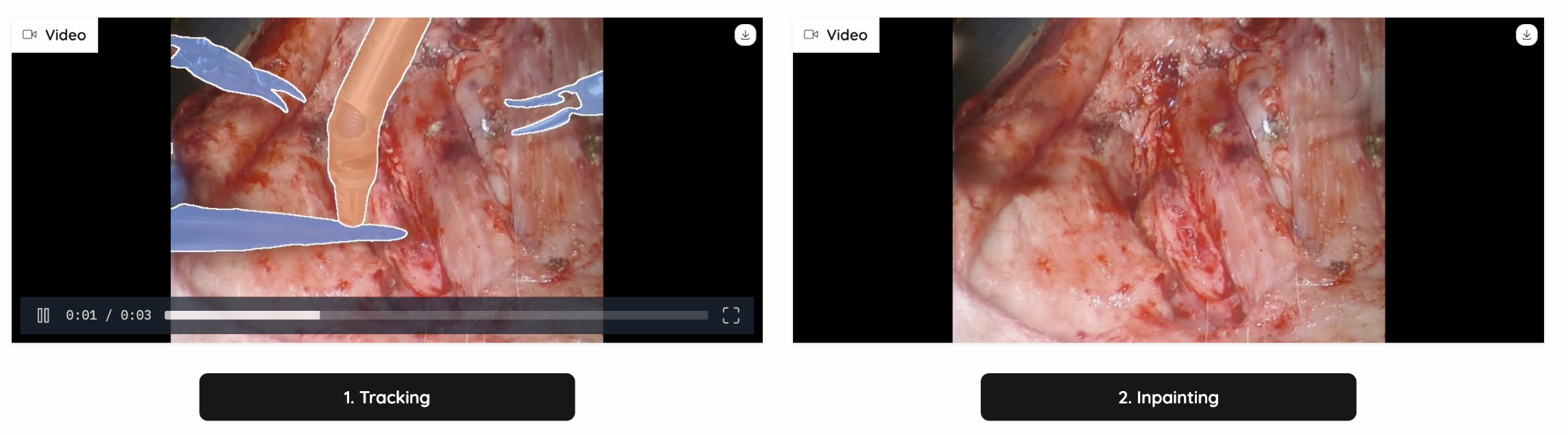
Figure 7: Inpainting Example 1
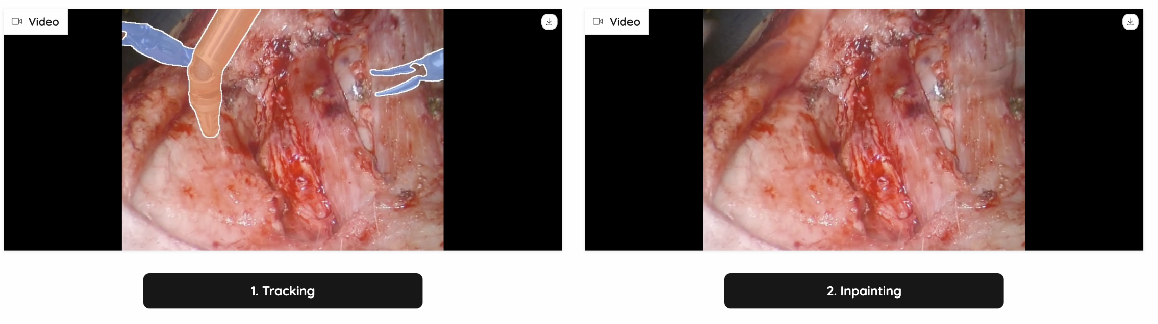
Figure 8: Inpainting Example 2
Text Prompt for SAM2 Input
To automate the whole process, we chose YOLOv8 (You Only Look Once v8) to provide input to SAM2. YOLOv8 is the latest version of the YOLO family, a state-of-the-art real-time object detection model developed by Ultralytics. It improves upon its predecessors by incorporating advanced deep learning techniques for better accuracy, efficiency, and versatility across multiple computer vision tasks.
However, YOLOv8 is not designed for unusual items such as medical instruments. Thus, we chose CholecT50 (Cholecystectomy Action Triplet) introduced by Nwoye et al. in Rendezvous: Attention Mechanisms for the Recognition of Surgical Action Triplets in Endoscopic Videos as our finetuning dataset. CholecT50 contains 50 endoscopic videos of laparoscopic cholecystectomy surgery introduced to enable research on fine-grained action recognition in laparoscopic surgery. It is annotated with triplet information in the form of <instrument, verb, target>. Due to the length constraints of this blog, we will not delve into the fine-tuning details. However, if you intend to provide text prompts to ProPainter, we recommend fine-tuning YOLO or your chosen model first.
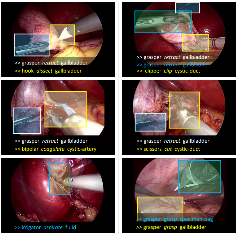
Figure 9: CholecT50 Dataset Example
Solutions for Blurriness
For medical instruments inpainting, the outcome of ProPainter is satisfying. However, the outcome of inpainting homorrage can be very blurry as shown below:
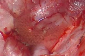
Figure 10: Example of Blurriness
Our First Trial: Propainter Reference Selection Optimization
To improve the blurriness of the inpainted area, we provide several intuitions for modifying the reference image list and neighbor list.
Since we found that these surgical videos tend to have more blood when it reaches the end of the video, we limited the reference selection range to “only the frames in the past“. This will lead to another advantage of testing the possibility of real time inferencing during the doctor’s sugery.
We defined a parameter K, and calculate the K value for every frame.
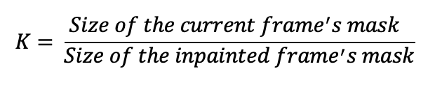
For every frame, we calculate its K value. For any frame that has a K value exceeding a pre-defined threshold T, we search with stride of N and replace them with the best search result, while preserving the chronological order. The parameter Stride N and Threshold T can be tuned for a better inference outcome.
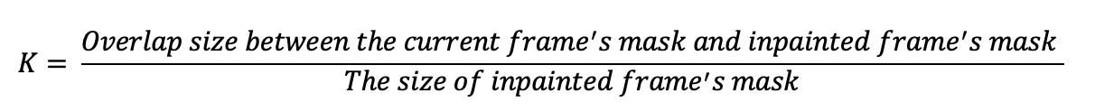
Considering the specific type of videos we are dealing with, we found that the surgical videos tend to move slow. Even if the mask is big in a certain frame, it still may provide more information because the mask is in such a different area. Thus, we re-defined the parameter K with the following equation:
Our Second Trial: Filtering in the Spatial Frequency Domain
Intuition:
We have tested several deblur models, but they were not performing well on surgical images due to a lack of training data. Considering that our video contains a lot of frames, the processing time of using these models would be long and inefficient.
Thus, we decided to rely on FFT’s ability to quickly transform an image from the spatial domain (where pixel intensity is directly represented) to the spatial frequency domain (where patterns, edges, and structures are represented as combinations of 2D-sinusoids at different frequencies).
In the spatial domain, sharp edges and fine details correspond to high-frequency components. Deblurring can be seen as the operation of enhancing the high spatial frequencies while attenuating the lower spatial frequencies. The filtering could be done in the spatial domain directly using convolution, but the process of designing the required filter would be complex, and the computing time at inference would be higher. In the spatial frequency domain, the filter design is simple and will look like a 2D ellipsoid of which the steepness of the slope will be chosen empirically.
Application Details:
Step 1: Read the input image as an RGB image and split the image into three channels. We read the mask as a grayscale image where 0 indicates a single channel.
Step 2: We compute the sum of masked channel pixel values (for the normalization needed at a later stage) and apply a 2D-FFT to each channel to transform it into the frequency domain.
Step 3: Define a function to create a 2D Gaussian-like frequency filter mask.
-
Iterate over all pixels in the frequency domain.
-
Compute the mask value based on Gaussian decay and scaling factors for different quadrants.
Frequency Filter for Deblur
sigma = 20
K2 = 0.66
K3 = 0.7
image_shape = (480, 640)  # Adjust if your image dimensions differ

def create_filter_mask(shape, sigma, K2, K3):
    """Create a Gaussian-like 2D filter in the spatial frequency domain."""
    rows, cols = shape
    mask = np.zeros((rows, cols))

    for n in range(rows):
        for m in range(cols):
            if n < 240 and m <320:
                mask[n, m] = (1 - K3 * np.exp(-((n) ** 2  +
                                             (m ) ** 2 )/ sigma ** 2)) ** K2
            if n < 240 and m >= 320:
                mask[n, m] = (1 - K3 * np.exp(-((n) ** 2  +
                                             (m - cols+1) ** 2 )/ sigma ** 2)) ** K2
            if n >= 240 and m <320:
                mask[n, m] = (1 - K3 * np.exp(-((n - rows +1) ** 2  +
                                             (m ) ** 2 )/ sigma ** 2)) ** K2
            if n >= 240 and m >= 320:
                mask[n, m] = (1 - K3 * np.exp(-((n - rows +1 ) ** 2  +
                                             (m - cols+1) ** 2 )/ sigma ** 2)) ** K2
    return mask
filter_mask = create_filter_mask(image_shape, sigma, K2, K3)
To accomplish this, we need to define parameters for the spatial cutoff frequency and filtershape:sigma (spread), K2 and K3 (scaling constants). These three parameters define the cutoff frequency and the shape of the 2D filter.
Step 4: Apply filter mask.
Now we created the filter mask for the given image dimensions and parameters. For all three channels, we transform them to the frequency domain, multiply them by the generated frequency mask, and apply inverse 2D-FFT to transform the filtered data back to the spatial domain and only extract the real part of the transformed data.
Apply Mask and Inverse FFT
F_r = fft2(red_channel)

# Step 2: Apply frequency filter mask
F_filtered_r = F_r  * filter_mask

F_inverse_r = ifft2(F_filtered_r)
F_real_r = np.real(F_inverse_r)

# Do the same steps for F_g and F_b
Step 5: Rescale the image.
Compute the maximum pixel value across all channels and normalize each channel by scaling pixel values to [0, 255] using the maximum color.
Rescaling
max_b = np.max(F_real_b)
max_g = np.max(F_real_g)
max_r = np.max(F_real_r)
max_color = np.max([max_b,max_g,max_r])

F_n_b = F_real_b* 255/ max_color
F_n_g  = F_real_g* 255/ max_color
F_n_r  = F_real_r* 255/ max_color
Step 6: Adjust the masked region.
Sum of Original and Filtered Masked Region
sum_r_0 = np.sum((mask/255) * red_channel)
sum_g_0 = np.sum((mask/255) * green_channel)
sum_b_0 = np.sum((mask/255) * blue_channel)

sum_r_1 = np.sum((mask/255) * F_n_r)
sum_g_1 = np.sum((mask/255) * F_n_g)
sum_b_1 = np.sum((mask/255) * F_n_b)

def clip(matrix):
    """Clip pixel values to the [0, 255] range."""
    matrix = np.where(matrix > 255, 255, matrix)
    matrix = np.where(matrix < 0, 0, matrix)
    return matrix

F_normal_b= clip( F_n_b * sum_b_0 / sum_b_1)
F_normal_g= clip(F_n_g * sum_g_0 / sum_g_1)
F_normal_r= clip (F_n_r * sum_r_0 / sum_r_1)
We try to preserve the relative brightness and intensity balance in the masked region after filtering. Without this adjustment, the filtered region will likely appear too dark or too bright, with a change in the balance of colors compared to the original image, causing inconsistencies.
To achieve this purpose, we first recalculate the sums of original and filtered channel values within the masked region. Then, we normalize the filtered red channel using the ratio of original to new masked sums, which actually serves as a scaling factor: If sum_r_1 is smaller than sum_r_0, the scaling factor increases the intensity values of the filtered region. Conversely, if sum_r_1 is larger, it reduces the intensity values.
However, we noticed that after the normalization, the value of some pixels may exceed the range of [0,255]. Thus, we defined the Clip function to ensure no display error will occur due to the values that are out of range.
Step 7:
Since the blurriness only appears in the inpainted area, we do not want to apply our deblur technique on other regions. The following code will help us combine original and filtered channels selectively, applying the filtered channel (M3) only within the masked region(M2). We will reconstruct the RGB image with a better result.
Only Filter for Inpainting Region
def mix(M1, M2, M3):
    """Only filter the inpainting region."""
    result = np.where(M2 == 255, M3, M1)
    return result

final_b = mix(blue_channel, mask, F_normal_b)
final_g = mix(green_channel, mask, F_normal_g)
final_r = mix(red_channel, mask, F_normal_r)

final_image = cv2.merge([final_r, final_g, final_b]).astype(np.uint8)

filter_image = cv2.merge([F_normal_r, F_normal_g, F_normal_b]).astype(np.uint8)
Here is an example of our deblur method’s effect:
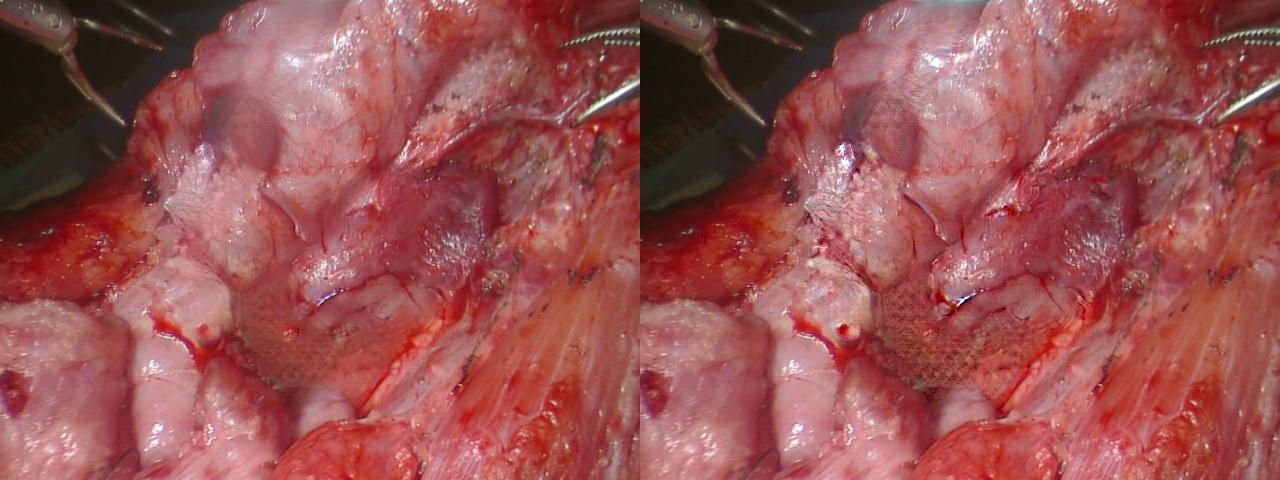
Figure 11: Deblur Method Effect
Measurements on the Images
Background
Can we extract precise measurements from surgical videos? To what degree of accuracy? Can we determine movement along the z-axis? For instance, could we measure the three-dimensional displacement of a surgical tool?
In the video, the primary surgical instrument in focus is a suction tool used to remove blood. Our SAM2 model provides a segmentation contour for this instrument. The first fundamental question is: “How precise is this contour?” To assess the measurement accuracy achievable with our model, we designed and conducted an experiment.
Experimental Setup
To evaluate contour precision, we conducted a simple experiment:
1. We selected four images and generated eight variations of each by applying a combination of transformations, including:
- Rotation
- Translation (shift)
- Scaling
- Horizontal flip
- Minor color balance adjustments
2. Each modified image was processed through SAM2, generating eight segmentation contours per original image.
If SAM2 were perfectly precise, these eight contours would be identical. While we know this will not be the case, analyzing the variation among these contours allows us to quantify the model’s segmentation accuracy.
Measurement Methodology
Using only a single point or a few points from a contour would lead to higher measurement variability, with precision in the range of multiple pixels. However, leveraging as many contour points as possible results in an averaging effect, improving precision according to the square root of N rule.
To estimate an upper bound on measurement precision, we computed the center of gravity of the contour, correcting for any scaling or shifts by using all contour points. We then performed linear regression on the tool’s contour edges to estimate the diameter of the tool handle.
Results & Conclusion
Repeating this process across eight images, we computed the standard deviation of the diameter measurements, leading to an estimated precision of approximately 0.5 pixels (the mean standard deviation across all eight sets).
Our conclusion is that SAM2’s contours exhibit a high degree of precision, making them reliable for measuring surgical tool dimensions with sub-pixel accuracy.
Displacement of the Surgical Tool
To estimate the displacement of the surgical tool, we will analyze its movement in both the x,y plane and along the z-axis.
-
x, y Plane Displacement:
- We will calculate the pixel displacement of the tool relative to its position in the first frame of the video.
- This displacement value will be displayed in the upper left corner of the video for each frame.
- Additionally, we will mark the initial reference point on the tool with a large yellow dot to visually indicate the tracked position.
-
z-axis Displacement
- The displacement along the z-axis will be inferred from changes in the apparent diameter of the tool.
- A positive value will indicate movement toward the viewer, while a negative value will indicate movement away from the viewer.
- This measurement will be the second number displayed in the video.
To obtain precise displacement values in pixels or millimeters, additional information about the camera optics would be required. However, for the purposes of this analysis, such calibration is not yet necessary.
The Algorithm
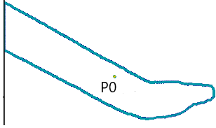
1. Compute the Contour’s Center of Gravity (P0)
We extract the tool’s segmentation contour from the image and remove contour regions at the image boundaries to ensure a large enough visible portion of the tool remains. Now we can compute the center of gravity (P0) of the contour, which should ideally be inside the handle of the tool.
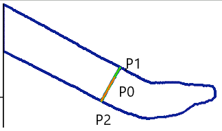
2. Identify the Closest Contour Point (P1) on One Edge
- From P0, draw a vertical line downward (the x-axis points toward the bottom).
- Decrease the x-coordinate in small increments, rounding to the nearest pixel.
- Stop when encountering a contour pixel, marking this P1.
- Repeat this process across angles from 0° to 180° to determine the angle that minimizes the distance to the contour, ideally perpendicular to the tool’s edge.
3. Find the Opposite Edge (P2)
- From P1, search for the opposite edge by rotating 180° from the optimal angle found in Step 2.
- Adjust the search range within ±5° to refine the position of P2 on the opposite contour.
4. Compute the Tool’s Midline
- Draw L1, the line connecting P1 and P2 (representing the tool’s width).
- Compute the midpoint P3 of L1.
- From P3, draw L2, a perpendicular line to L1 (representing the estimated tool axis).
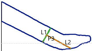
5. Find the Tool’s Tip
- Identify P4, the intersection of L2 with the contour near the tool tip.
- Increment x along L2, checking if a new line L3 (parallel to L1) intersects the contour.
- If an intersection is found, repeat the process. If not, the tip of the tool is located.
- Retract 150 pixels (normalized to P1-P2 distance) along L2 to define P5.
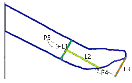
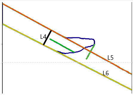
6. Define Tool Orientation and Edge Regression
- From P5, draw L4, a line parallel to L1, dividing the space into four quadrants.
- Extract the two straight edge contours of the tool.
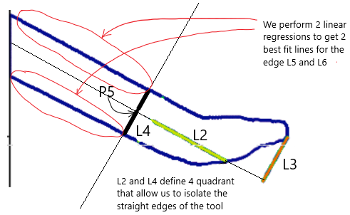
- Perform linear regression on these contours to obtain L5 and L6, refined approximations of the tool’s edges.
- Compute the average slope of L5 and L6, defining a new line L7, which passes through P6 (midpoint of L4’s intersections with L5 and L6).
- Construct L8, the perpendicular to L7 at P6.
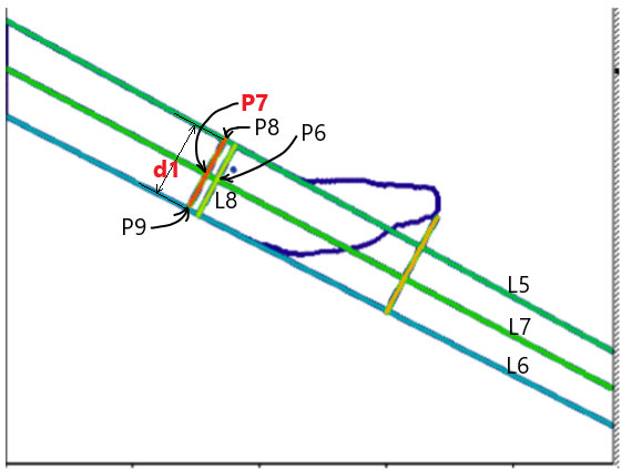
7. Refining the Tool Displacement Measurement
- Repeat Steps 4-6, replacing P3 and L1 with P6 and L8, to compute a new P7.
- Using P7 and L7, determine L9, the refined midline.
- Find the intersections of L9 with L5 and L6, defining P8 and P9.
- Compute the midpoint P7 between P8 and P9, which serves as the tool displacement measurement point.
- The variation in distance d1 (between P8 and P9) provides an estimate of the tool’s displacement along the z-axis.
To accurately track the surgical tool, the algorithm ensures precise edge detection by using small incremental steps when adjusting the x-coordinate. Both the x and y increments are constrained to ≤ 0.5 pixels, preventing the algorithm from skipping over thin tool edges, which can be as narrow as a single pixel. This fine-grained step size guarantees that the edge detection process remains accurate, particularly in cases where the tool contour is only a few pixels thick.
To further reduce noise in the measurements, an exponential moving average is applied to several key parameters: the tool axis angle, the estimated tool diameter (d1), and the coordinates of the “yellow dot” (P7). This smoothing technique enhances the stability of measurements over consecutive frames. However, when the center of gravity (P0) shifts by more than 5 pixels between frames, the averaging process is reset to prevent outdated values from affecting new measurements. This ensures that motion is tracked with high precision while minimizing the impact of noise when the tool remains relatively stable.
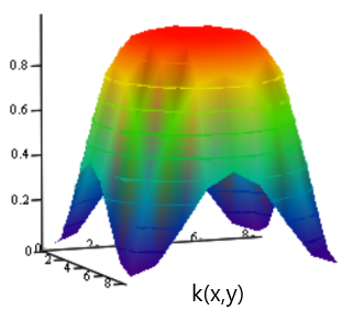
Visual Representation of P7 in the Video
The representation of the point P7 in the video is done using a 2D function centered on the floating point coordinates (x,y) of P9. To render the dot accurately within the pixel grid, the function values k(x,y) are computed as samples of the 2D function at the integer pixel coordinates of the image. These function values are then blended with the existing pixel intensities in the image to ensure a smooth transition.
The blending process follows the formula:

wherek(x,y) controls the weighting between the generated point and the original image content. To ensure clear visibility, the dot size is set to 9 pixels in diameter. The 2D function defining the intensity distribution is given by:
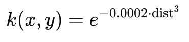
where dist represents the pixel distance from the function’s peak intensity. The function values range between 0 and 1, ensuring a gradual and natural blending effect with the surrounding pixels, resulting in a smooth, visually distinguishable representation of P7 in the video.
The example video will provide two synchronized videos side by side, showing the before and after inpainting, with contours indicating the targeted areas.
You can check out our final UI video here.
References
-
Kirillov, Alexander, et al. “Segment Anything.” Proceedings of the IEEE/CVF International Conference on Computer Vision. 2023.
-
Miao, Albert J., et al. “Hemoset: The first blood segmentation dataset for automation of hemostasis management.” 2024 International Symposium on Medical Robotics (ISMR). IEEE, 2024.
-
Ravi, Nikhila, et al. “SAM 2: Segment Anything in Images and Videos.” arXiv preprint arXiv:2408.00714 (2024).
-
Reis, Dillon, et al. “Real-Time Flying Object Detection with YOLOv8.” arXiv preprint arXiv:2305.09972 (2023).
-
Zhou, Shangchen, et al. “Propainter: Improving propagation and transformer for video inpainting.” Proceedings of the IEEE/CVF International Conference on Computer Vision. 2023.