A simple machine learning model’s performance would largely tie throughput to the FLOPS of the system. However, host interactions may notably affect performance, such as tensor data transferred in and out of the device or post-processing interleaved between inference steps. Having a good understanding of such interactions is paramount to reduce execution time.
In the quest of optimizing performance, trace visualization apps are a very powerful tool to analyze interactions between layers of software and the accelerator, allowing us to easily locate inefficiencies happening during inference execution.
For that matter, ONNXRuntime provides easy-to-use parameters to enable execution event tracing. In a transparent way, the ET-SoC-1 provider extends tracing to also include detailed backend, runtime and device events. As a result, without additional parameters or API calls, we will obtain a single timeline containing all-component events happening during execution.
This blog post has two objectives. First, we show how to enable traces when running models with ONNXRuntime and how to visualize them. Second, we show how to profit from the information in the screen to find performance issues and opportunities for optimizations.
Let’s see how it is done.
Enabling and Visualizing Traces
First of all, to enable profiling traces for your own ONNXRuntime ML scripts, it is as simple as using the ONNXRuntime API and setting enable_profiling to true. This flag is agnostic to the platform and available no matter which backend is used. Example below for Python:
import onnxruntime
sess_options = onnxruntime.SessionOptions()
# Pick a trace filename prefix
session_options.profile_file_prefix = f'yourmodel_etglow_window_1'
# Enable tracing in Session options
session_options.enable_profiling = True

# Then, run your inference
session_etglow = onnxruntime.InferenceSession(model, sess_options=session_options, providers=['EtGlowExecutionProvider'], provider_options=[provider_options])
Example
Following this, we will provide a brief introduction on the kind of information that we can infer from an execution trace when running a model.
For this example, we will use the script that runs LLM networks with KV-Cache optimizations enabled, as shown in our previous post.
Generating the Trace
To generate the trace, simply just run your code. A .json trace file will be placed in the current working directory. In our case, it looks like this:
-rw-r--r-- 1 user eng 46M Oct 18 11:32 llama3-8b-instruct-kvc-int4_etglow_window_1_2024-10-18_11-24-17.json
Opening the Trace File in Perfetto
The perfetto visualization tool is available online: ui.perfetto.dev
To open a trace, navigate to the perfetto website and drag and drop the .json trace file previously generated. If the trace was generated properly, a similar screen will appear:
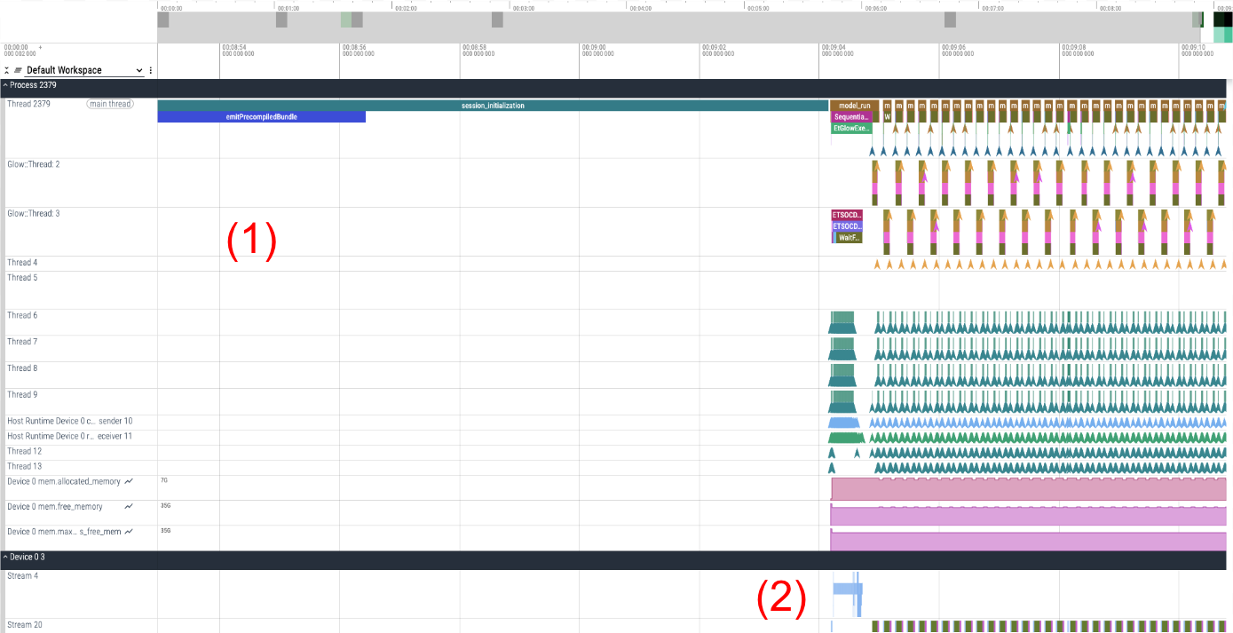
Figure 1
In the trace above, we find two groups of rows. These rows usually map to threads or streams. From now on we will refer to these as tracks. The (1) group corresponds to rows containing events happening in the host side, whereas tracks in group (2) contain events happening in the device.
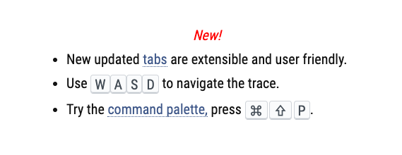
Main controls are shown in the main screen before loading any trace. The mouse cursor can also be used to aim for the region you want to zoom in to very fast, which is a nice feature.
Analyzing the Trace
Step 1: Regions of Interest
To run an inference, there is a previous initialization phase where the model network and weights are loaded into the device – this cost is paid once and split between session_initialization (3) and the first inference (4).
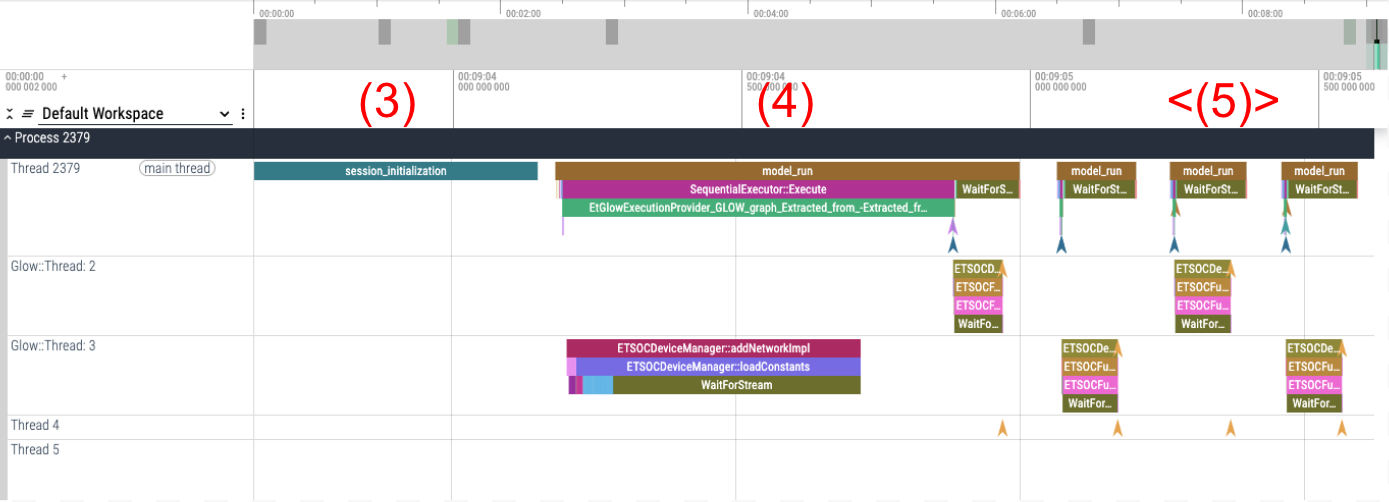
Figure 2
The rest of the inferences have a steady execution time per inference (5), which compose our region of interest.
Step 2: Finding the Tracks of Interest
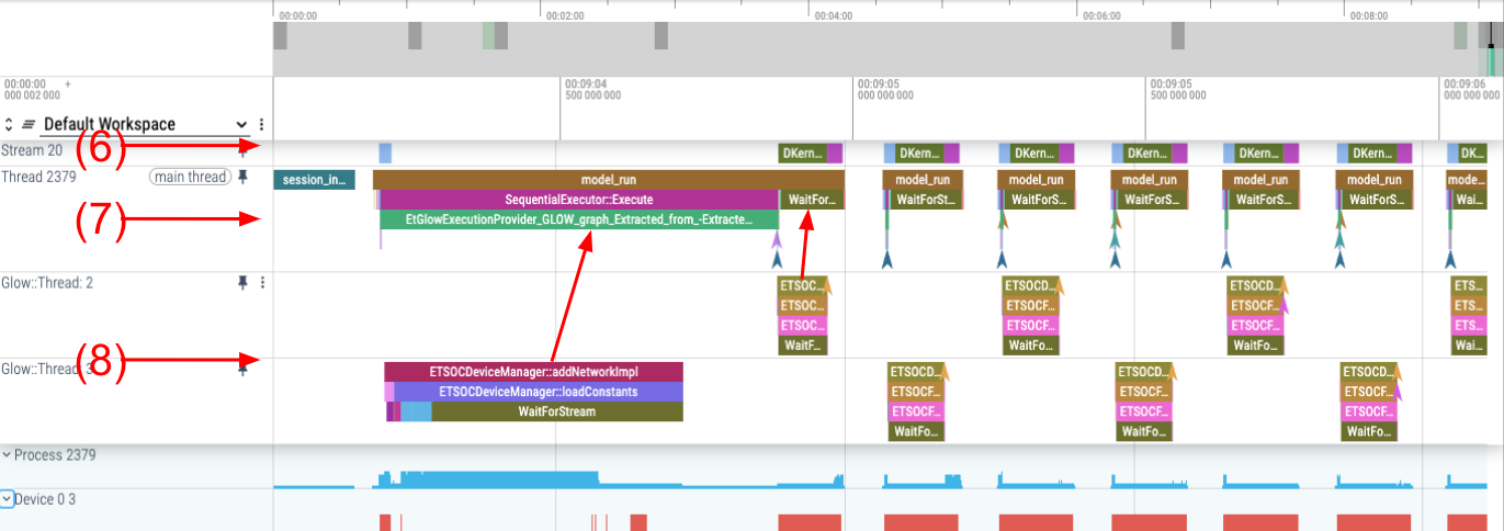
Figure 3
To have a less convoluted view of what is happening during execution, we recommend starting by pinning a few relevant tracks for an easy first analysis:
-
The streams containing DKernel executions in the Device track group (6).
-
The main_thread in Process (7).
-
The threads labeled Glow::Thread <X> containing events with name prefix ETSOC (8).
Basic Interactions: Examples
One example where we can see how it helps to have events happening in multiple layers of software under the same timeline is the area with two arrows pointing to the model run event in the main thread in Figure 3. As we see, the total inference time, represented by model_run, is significantly longer than the rest following. Using the current view, we can easily connect event dependencies causing this issue. In this case, the ETSOCDeviceManager::loadConstants call to load the weights that is required the first time a network runs is causing this longer execution.
Step 3: Analyzing the Region of Interest
Ideally, the computational part of the model should dominate the execution time. Therefore, one of the first goals that we can set analyzing a trace is to see what is taking time away from that computational part.
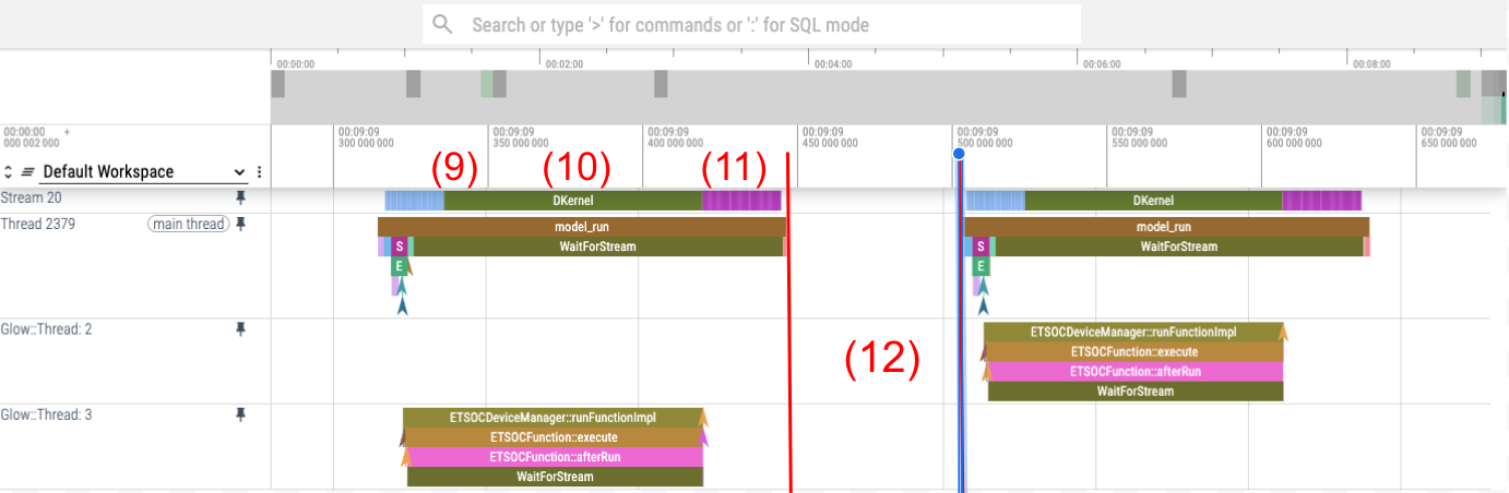
Figure 4
If we focus on the region of interest shown in Figure 4, we can quickly locate the data transfers going from the host into the device (9), the inference execution, DKernel (10), and data transfer back to the host (11). Inside each inference (model_run) taking 135ms, we spend roughly 36% (49ms) of the time moving data. In addition, there is a gap of ~40ms between iterations without tracing events.
Now, if we want to proceed further with optimizations, we must revisit the code we are running to understand if the time used for non-compute tasks can be avoided or not. In this particular case, we found out two interesting pieces of information. First, (10) and (11) correspond to unnecessary copies back and forth of the KV-Cache tensors, and second, the gap between inferences (12) is spent doing sequential post-process. In a follow-up blog post, we are going to show we can avoid such unnecessary copies with ONNXRuntime I/O Bindings and greatly improve performance.
Conclusion
With very easy-to-use tools, we were able to see a visual overview on where the model spends the CPU and ET-SoC-1 cycles. This allowed us to quickly understand possible sources of issues with data transfers and post-process in our script running KV-Cache enabled LLMs to process questions and generate answers.